5Week 40

5.1 Readings for this week's lectures

Sections 15.1-15.2 in the textbook.

5.2 Readings for this week's exercises

Sections 14.2-14.3 og 14.6 in the textbook.

5.3 Notes

Partial differentiation

If $z=f(x,y)$ , then:

$\frac{\partial z}{\partial x} = f'_x(x,y) = f'_1(x,y) = \text{the partial derivative of~} f(x,y) \text{~with respect to~} x.$

$\frac{\partial z}{\partial y} = f'_y(x,y)=f'_2(x,y) = \text{the partial derivative of~} f(x,y) \text{~with respect to~} y.$

To take the partial derivative with respect to a variable, consider the other variable as a constant. We can, temporarily, consider $f$ a function of one variable. Example: To find $\frac{\partial z}{\partial x}$ : think of $y$ as a constant and differentiate $f(x,y)$ as if $f$ only depended on $x$ .

5.4 Problems

Drag expressions from the boxes at the bottom into the empty boxes, so that the equations are correct.

$f'_x(x,y) =$

$\frac{\partial z}{\partial y} =$

$f''_{xy}(x,y) =$

$f''_{yy}(x,y) =$

$\frac{\partial^2 f}{\partial x\partial y}$

$\frac{\partial^2 f}{\partial^2 y}$

$\frac{\partial f}{\partial x}$

$z'_y(x, y)$

$\frac{\partial^2 f}{\partial y^2}$

$\frac{\partial^2 f}{\partial y\partial x}$

$z'_1(x, y)$

A function $z = f(x,y)$ is defined by:

$z=f(x,y) = 3x^5 + 4y^2-8xy$ Find:

$\frac{\partial z}{\partial x}$
$\frac{\partial z}{\partial y}$
$f'_1(-1,1)$
$f'_2(-1,-1)$

A function $z = f(x,y)$ is defined by:

$f(x,y) = \sqrt{x^2+y^2}$ Find:

$f'_1$
$f'_2$
$f'_1(-2,-8)$
$f'_2(3,7)$

For the function $f(x,y)=e^{8xy}$ , find $f'_x$ and $f'_y$ .

Consider a production function $Y = F(K, L)$ , where $K$ is units of capital and $L$ is units of labour. $Y$ is the number of produced units.

Connect the statements below with the correct mathematical expressions, by dragging the mathematical expressions on to the correct boxes.

a) With 10 units of capital and 25 units of labour, 5 units can be produced

b) With 10 units of capital and 25 units of labour a small increase in units of labour will give approximately 2 extra produced units per unit of labour

c) The more units of labour, the greater the effect on production from an extra unit of capital

$F_K'(10,25)=5$

$F(10,25) = 5$

$F_{KL}''(K,L)<0$

$F_K'(10,25)=2$

$F_K'(K,10) > F_K'(K,15)$

$F(25,10)=5$

$F_{KL}''(K,L) > 0$

$F_L'(10,25)=2$

For the function $f(x,y)=x\ln(4x+y)$ , find $f'_x$ and $f'_y$ .

Find $\frac{\partial z}{\partial y}$ if $z = 2(8x+4y)^3$

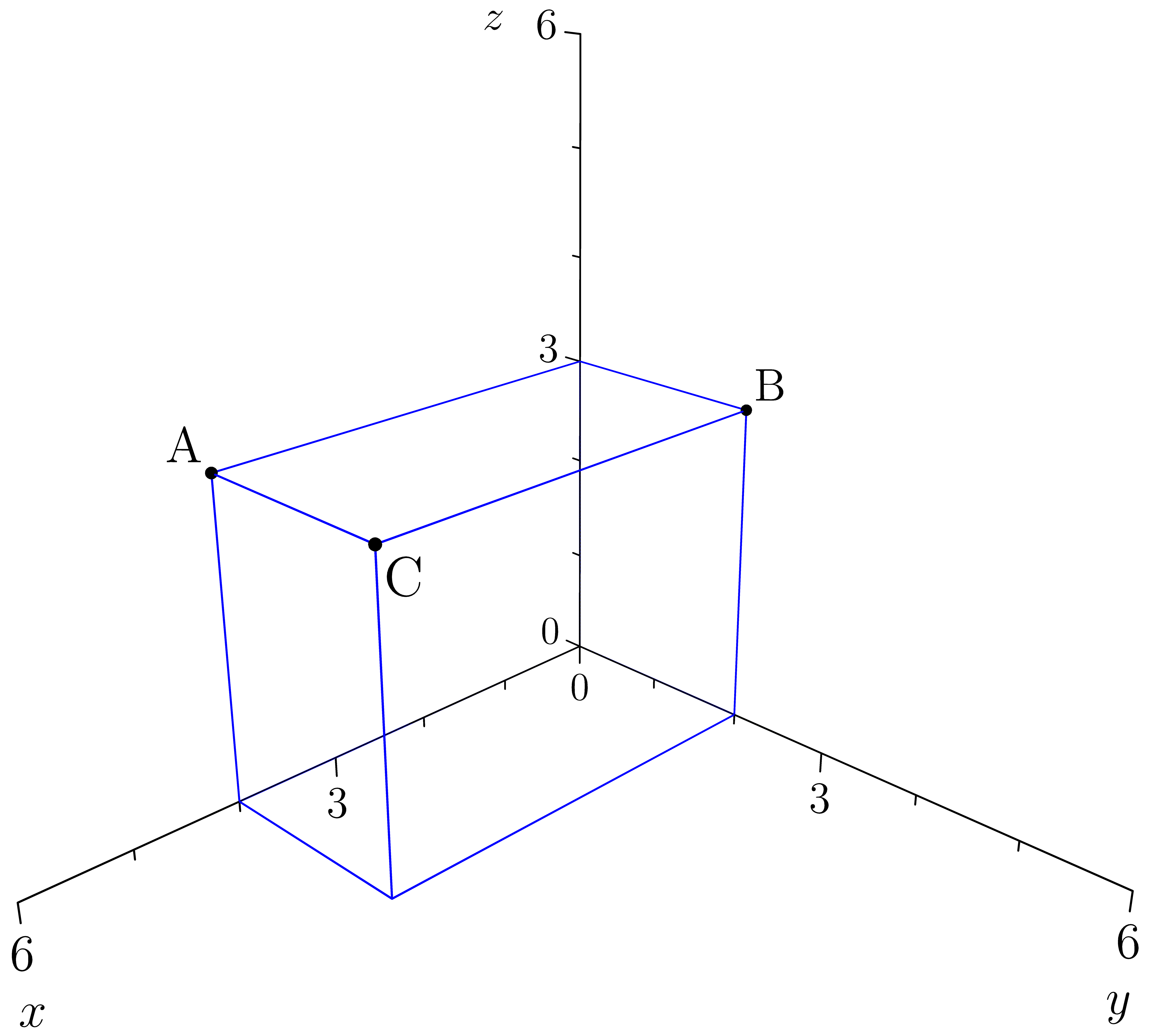
Find the coordinates of the points A, B and C of the box shown below.

Below are shown three level curves for a function $z=f(x,y)$ . For each level curve, the value of $z$ is shown above the curve.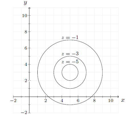

Determine $f(1,3), f(6,3), f(5,5)$ and $f(5,-1)$
Solve the equations $f(4,y)=-5$ and $f(x,3)=-1$
Find approximations to $f_x'(6,3)$ and $f'_y(5,4)$

A function has the contour plot shown below, where the level curves are equally spaced in $z$ .

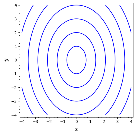
Which of the following functions is shown in the contour plot? Explain how you got the answer.

Eliminate options by considering the answers to the following two questions:

The level curves lie at a fixed distance along a given line through $(0,0)$ , e.g., the $x$ -axis or the $y$ -axis. What does that imply?
In which direction does the function grow fastest? You can determine that by looking at the distance between the level curves.

$x^2 + 2y^2$

$\sqrt{x^2 + 2y^2}$

$2x^2 + y^2$

$\sqrt{2x^2 + y^2}$

Below are shown contour plots for some functions. Match each plot with the correct function. The blue lines are the level curves for $z = 0$ .

Consider the solution to $f(x, y) = 0$ which corresponds to the blue curves in the plots.

Function 1:

Function 2:

Function 3:

Function 4:

$2(x^3 - y^3) \Big/ 3\sqrt{x^2 + y^2}$

$xy$

$x^2 - y^2$

$2(x+y)$

Consider the function defined by

$z=\frac{1}{3}\left ( x^2+y^2 \right )$ Sketch the level curve for $z=c$ where $c=0,1,2,3,4$ .

Determine the level curve for the function $f(x,y) = \sqrt{30-x^2-y^2}$ at the value $c=5$ and sketch the curve.

For the function $f(x,y,z)=8+2xy^4-5z^5$ , find $f'_1$ , $f'_2$ and $f'_3$ .

Let

$f(x,y,z)=\frac{9+x^2y^4}{z^3}$ Find $\frac{\partial f}{\partial x}$ , $\frac{\partial f}{\partial y}$ , and $\frac{\partial f}{\partial z}$

This exercise shows an example where Young's theorem does not hold. You are not required to go through this, but it is provided to those interested.

Consider the function $h(x, y) = \frac{{\left(x^{2} - y^{2}\right)} x y}{x^{2} + y^{2}}$ , which is plotted below.

The only apparent problem with $h(x)$ is that it is not defined at $(x, y) = (0, 0)$ . But the limits as $x\to 0$ and $y\to 0$ exist:

$\begin{aligned} \lim_{x\to 0} h(x, 0) & = 0 \\ \lim_{y\to 0} h(0, y) & = 0 \end{aligned}$

We can therefore define a function that is continuous for all $(x, y)$ including $(0, 0)$ as follows:

$f(x,\,y) = \begin{cases}{\frac {xy\left(x^{2}-y^{2}\right)}{x^{2}+y^{2}}}&{\text{ for }}(x,\,y)\neq (0,\,0),\\0&{\text{ for }}(x,\,y)=(0,\,0).\end{cases}$

Taking the partial derivatives of $f(x, y)$ is straightforward, but rather tedious. If you wish, you can verify that the two first-order partial derivatives are:

$\begin{aligned} f'_x(x, y) & = \frac{2 \, x^{2} y}{x^{2} + y^{2}} - \frac{2 \, {\left(x^{2} - y^{2}\right)} x^{2} y}{{\left(x^{2} + y^{2}\right)}^{2}} + \frac{{\left(x^{2} - y^{2}\right)} y}{x^{2} + y^{2}} \\ f'_y(x, y) & = -\frac{2 \, x y^{2}}{x^{2} + y^{2}} - \frac{2 \, {\left(x^{2} - y^{2}\right)} x y^{2}}{{\left(x^{2} + y^{2}\right)}^{2}} + \frac{{\left(x^{2} - y^{2}\right)} x}{x^{2} + y^{2}} \end{aligned}$

Show that $f'_x(0, y) = -y$
Show that $f'_y(x, 0) = x$

Now, we can compute the second order derivatives in the point $(0, 0)$ as:

$\begin{aligned} f''_{xy}(0, 0) & = \frac{\partial f'_x(0, y)}{\partial y} (0, 0) \\ f''_{yx}(0, 0) & = \frac{\partial f'_y(x, 0)}{\partial x} (0, 0) \end{aligned}$

Calculate $f''_{xy}(0, 0)$ and $f''_{yx}(0, 0)$ is indicated above.
What can you conclude?