10Week 45

10.1 Readings for this week's lectures

Sections 10.1-10.4 in the textbook.

10.2 Readings for this week's exercises

Sections 18.2–18.5 in the textbook.

10.3 Notes

The Lagrange multiplier method

To find a max/min for $f(x,y)$ under the constraint $g(x,y)=c$ ...

Construct ${\cal L} (x,y) = f(x,y) - \lambda \left( g(x,y)-c \right)$
Differentiate ${\cal L}$ wrt $x$ and $y$ and set ${\cal L}'_x = {\cal L}'_y = 0$ .
This gives the three equations:
${\cal L}'_1(x,y) = f'_1(x,y) - \lambda g'_1(x,y) = 0$
${\cal L}'_2(x,y) = f'_2(x,y) - \lambda g'_2(x,y) = 0$
$g(x,y) = c$
Solve these for $(x,y,\lambda)$ . These are the solution candidates.

Interpreting the Lagrange Multiplier

Let us denote the values solving the optimisation problem by $(x^*,y^*)$ . They are a function of $c$ , so we can introduce the function:

$f^*(c) = f(x^*(c),y^*(c))$

It turns out that (p. 739 in the textbook):

$\frac{df^*(c)}{dc} = \lambda(c)$ The interpretation of the above formula is that $\lambda$ is the growth rate of the optimised function when the constant $c$ in the constraint is increased. If $\Delta c$ is a small change in $c$ this means that

$f^*(c + \Delta c) - f^*(c) \approx \lambda(c) \Delta c$

$\lambda$ is thus marginal cost of the constraintor utility or profit, depending on what $f(x,y)$ describes. and also referred to as the shadow price.

Theorem 18.5.1 — global second order conditions

If $(x_0,y_0)$ is a stationary point for ${\cal L}(x,y) = f(x,y) - \lambda \left( g(x,y)-c \right)$ , then:

If ${\cal L}$ is concave, then $(x_0,y_0)$ is a solution to maximising $f(x,y)$ under the constraint $g(x,y)=c$ . That is:
$\frac{\partial^2{\cal L}}{\partial x^2} \leq 0, \qquad \frac{\partial^2{\cal L}}{\partial y^2} \leq 0, \qquad \frac{\partial^2{\cal L}}{\partial x^2} \frac{\partial^2{\cal L}}{\partial y^2} - \left[ \frac{\partial^2{\cal L}}{\partial x \partial y} \right]^2 \geq 0$
If ${\cal L}$ is convex, then $(x_0,y_0)$ is a solution to minimising $f(x,y)$ under the constraint $g(x,y)=c$ . That is:
$\frac{\partial^2{\cal L}}{\partial x^2} \geq 0, \qquad \frac{\partial^2{\cal L}}{\partial y^2} \geq 0, \qquad \frac{\partial^2{\cal L}}{\partial x^2} \frac{\partial^2{\cal L}}{\partial y^2} - \left[ \frac{\partial^2{\cal L}}{\partial x \partial y} \right]^2 \geq 0$

Theorem 18.5.2 — local second order conditions

Let $(x_0,y_0)$ be a stationary point for ${\cal L}(x,y) = f(x,y) - \lambda \left( g(x,y)-c \right)$ . With:

$\begin{aligned} D(x,y,\lambda) &= (f''_{11}-\lambda g''_{11}) (g'_2)^2 - 2(f''_{12} - \lambda g''_{12})g'_1g'_2\\ &+ (f''_{22}-\lambda g''_{22}) (g'_1)^2 \end{aligned}$

$D(x_0,y_0,\lambda) < 0$ : local solution to max. problem
$D(x_0,y_0,\lambda) > 0$ : local solution to min. problem

10.4 Problems

Consider the problem:

$\max f(x,y)=3x+4y$ s.t. $g(x,y)=x^2+y^2=225$ .

Solve both the maximization problem, but also the corresponding minimization problem. You may assume that a point with the highest function value is a solution to the maximisation problem and that a point with the lowest function value is a solution to the minimisation problem. Alternatively, you can use the local second-order conditions.
Suppose that the right-hand side of the constraint is changed from 225 to 224. What is the approximate change in the maximum value of $f$ ?

Allan wants to build a rectangular dog run with a certain length and width, and is interested in its area. He wants to use larch wood for the length and beech wood for the width. The cost of larch wood is 500 kr/m and the cost of beech wood is 250 kr/m. Allan has a budget of 10,000 kr for the dog run.

Introduce the needed variables and functions and formulate a maximisation problem with a constraint that corresponds to maximising the dog run under the constraints given by the price of the materials and Allan's budget.
Solve the problem and find the largest possible area of the dog run. You can assume that a maximum exists.
Allan regrets not allocating more money for the project. Assume that he had allocated 1000 kr more. Use your calculations in 2. and calculate, approximately, what the total area of the dog run would be with the bigger budget.
Allan is sceptical towards approximations, and prefer exact answers. If the budget were 11,000 kr, how big would the dog run have been?

The Cobb-Douglas production function for jeans is

$N(x,y)=60x^{0.8}y^{0.2}$ where $x$ is the number of units of labor with unit cost of 40 DKK, and $y$ is the number of units of capital with unit cost of 100 DKK. 500,000 DKK is budgeted for the production.

Determine how much of $x$ and $y$ should be allocated to maximize the production of jeans. You can assume that a maximum exists.

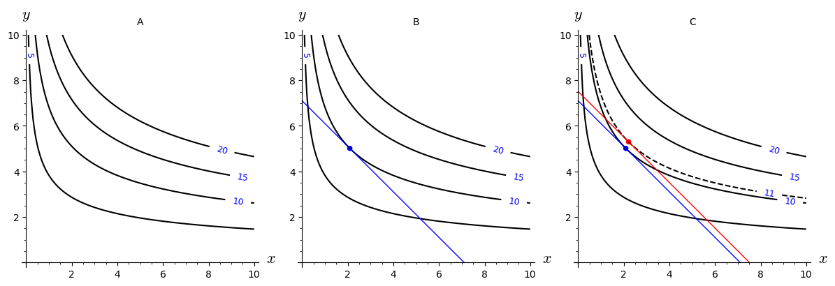
Figure A, below, shows the level curves for a function $f(x, y)$ . The value of the function is shown for each level curve. Use Figure A, B and C to answer the following questions:

Figure B shows the solution to an optimisation problem with the constraint $x + y = c$ , where $c = 7.1$ . Is the problem a minimisation or a maximisation problem?
Figure C shows a solution (in red) to the optimisation problem for a different value of $c$ . What value of $c$ does the solution correspond to?
What is the approximate value of $\lambda$ ?

Consider the function

$f(x,y) = 4xy$ and the constraint $x^2+y^2=8$ .

Find the critical points for the Lagrangian.
Determine the minimum and the maximum by calculating the function values in the critical points. You may assume that a point with the highest function value is a solution to the maximisation problem and that a point with the lowest function value is a solution to the minimisation problem (this is not generally the case).

Maximize $f(x,y)=10x^{1/2}y^{1/3}$ s.t. $2x+4y=10$ where $x\geq 0$ and $y\geq 0$ . Find the values of $x$ , $y$ and $\lambda$ that constitute the solution to the first-order conditions. You may assume that the solution solves the maximisation problem.

(Previous exam problem)

Consider the following mathematical problem:

$\min f(x,y)=x^2+y^2$ s.t. $10=x+y$ .

Solve the problem.
How can you know that you have not found a maximum point for the function $f(x,y)$ .

(Previous exam problem)

A function is given by

$f(x,y) = 10x+20y-(x^2+y^2)+50$

Find the stationary (critical) point for the function.
Characterise this point using a second-order test.
Solve the maximisation problem $\max f(x,y)$ under the constraint $g(x,y)=10$ , where $g(x,y)=x+4y$ .
Show that the point you found is a maximum and not a minimum.

(Previous exam problem)

A function of two variables $f(x, y)$ is given by the expression

$f(x, y) = xy^{\frac{2}{3}}, \quad x > 0, \, y > 0$

Find $x$ and $y$ that maximise the function under the constraint $g(x, y) = 2 x + 3 y = 2$ . You can assume that the point you find is a solution to the maximisation problem.
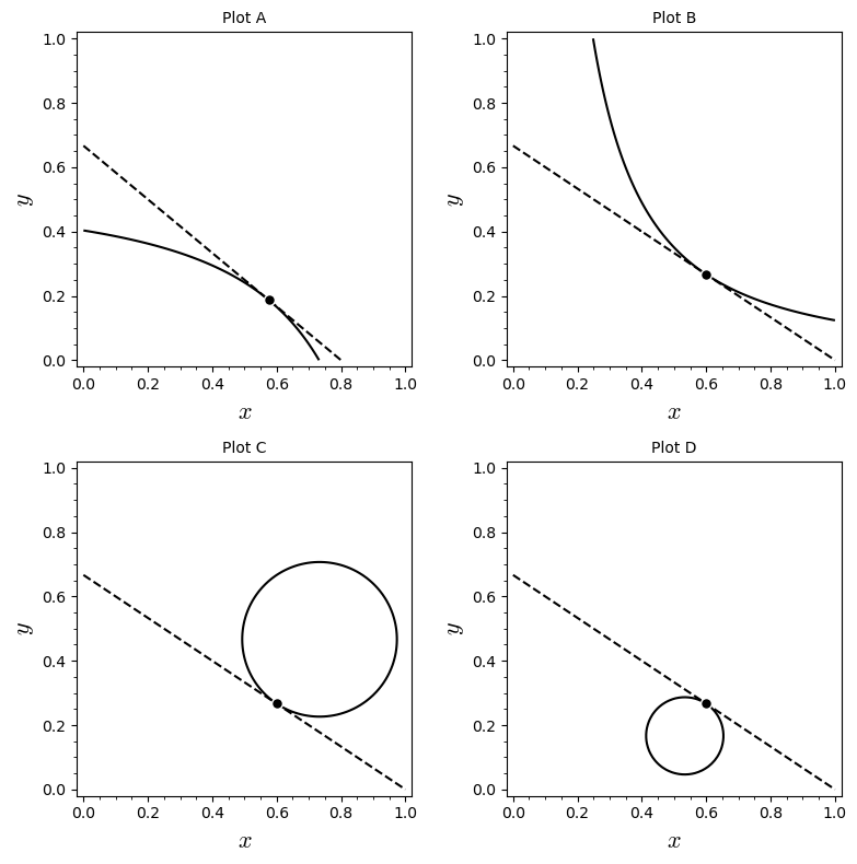
Which of the plots below illustrates the solution graphically? Give a brief explanation.